Retired Investor Model Portfolio Results from 2003 to 2019

The world of investment management is filled with backtests — the use of historical data to show how a proposed investment strategy or portfolio would have performed in the past. The problem is that this creates a strong temptation to tweak proposed strategies so that their backtests produce impressive results.

However, in a complex adaptive system like the global economy and financial market there is a strong likelihood that the future will not perfectly resemble the past. Put differently, in such systems it is often the case that the harder you try to fit your model to historical data, the less robust it will be to future uncertainties.

It is nonetheless interesting for investors to see how real, implemented strategies actually played out. Unfortunately, in this case the problem is "survivorship bias", which is a fancy way of saying that this type of historical analysis can lead to overoptimism and overconfidence because poorly performing strategies and funds are often killed off quickly, and disappear from data sets without leaving a long-term track record to examine.

Our time-out from publishing for a few years deprived us of the opportunity to quickly tweak our model portfolios had they not been working, or had we simply lost confidence in our methodology when financial markets hit hard times. We can therefore look at 16 years of historical data — from December 2003 to December 2019 — to see (warts and all) how our model portfolios actually performed.

Methodology

Our model portfolios were based on a regime switching model. We assumed that the financial markets could be in one of three regimes, that we termed normal times, high inflation, and high uncertainty. Based on our analysis of historical time series data, we estimated the probability that, conditional on being in one regime in a given year, the system would switch to one of the two others.

For each regime, we then estimated asset class inputs, including the average real return, standard deviation of return, and correlation with the real returns on other asset classes. To do this, we combined historical data with the outputs from our asset pricing model. Within each regime we assumed Gaussian/normal distributions of asset class returns. However, the different distributions within each regime and use of the regime switching model produced an aggregate distribution of asset class returns that was quite close to the distribution features observed in the historical data (i.e., fat tails, clustered volatility, etc.).

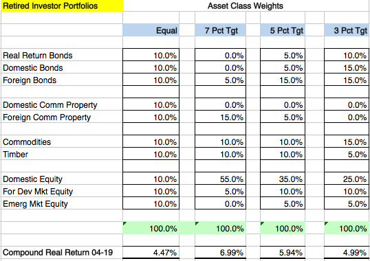
We used broad asset class definitions, and only included those classes for which retail index fund products were available at the end of 2003. These included (1) real return bonds; (2) domestic investment grade bonds (both government and credit); (3) foreign government bonds (without currency hedging); (4) domestic commercial property REITs; (5) foreign commercial property; (6) domestic equity (VTSMX); (7) foreign developed markets equity; (8) emerging markets equity; (9) commodities; and (10) timber REITS (which were more of a pure play on timber than paper and building products companies).

As we have previously noted, because of structural changes in the structure of the market for futures-based commodity index funds, we no longer believe that that broad-based commodity index products should be included in a portfolio. That said, because of what we believe to be long-term structural trends that favor relatively more upside surprises, we would consider narrower commodity index funds that track agricultural grains or industrial metals (except iron ore and aluminum).

In constructing our model portfolios, we also established certain constraints on maximum drawdown and allowable asset class weights, to avoid so-called "corner solutions" where almost all of a portfolio is allocated to one asset class.

Our models also sought to optimize rebalancing frequency to minimize risk and gain incremental return. This was accomplished by setting asset class portfolio weight thresholds that would trigger rebalancing (e.g., 10% above target weight) and when those occurred a target for incrementally overweighting the most underweight asset class or asset classes and underweighting the most overweight (to capture incremental returns from markets overshooting fair value in either direction).

For each long-term real return target (7%, 5%, and 3%), we employed simulation optimization to identify robust portfolios that maximized the probability of achieving the target within he constraints we set. These simulations included both the regime switching model and, within each regime, the range of possible returns on each asset class.

Our Benchmarks

We have judged the performance of our model portfolios against two benchmarks. The first is whether they have met their compound annual (i.e., geometric average) real return targets.

The second is how they compared to the results from an equally weighted mix of the broad asset classes we used.

To be clear, equal weighting implies that an investor has no confidence (beyond luck) in their ability to predict meaningful differences in future asset class returns, standard deviations, and correlations.

Put differently, it implies an investor has no confidence in their ability to predict future asset class exposures to the factors that drive returns (e.g., macroeconomic and investor behavior variables), and/or in their ability to predict the future returns associated with different degrees of exposure to those factors.

Model Portfolio Results

The following table shows the nominal return and standard deviation for our target return and equally weighted portfolios along with (a) the amount of return per unit of standard deviation; (b) the value at the end of December 2019 of an investment of 100 made at the end of December 2003; and (c) the compound real return (which can be compared to the portfolio target).

Please keep some caveats in mind when looking at these results:

• We do not adjust for annual management expenses charged on the funds whose results we track (assuming low cost index funds were used to implement our asset allocations, at the high end this could have reduced real returns by 0.50%. However 0.25% is probably more realistic.

• We assume constant asset allocation, and do not include the expenses associated with this rebalancing. Nor do we show the incremental impact of the model portfolio's systematic rebalancing strategy.

• Most important, we do not show the very substantial impact from what we call "episodic" rebalancing to avoid losses from substantial asset class overvaluations (e.g., our May 2007 warning that severe financial turbulence lay ahead, and our recommendation to move into cash).